
fitroom package
Submodules
Module contents
- class CaseSelector(dbInteractx=None, dbInteracty=None, xparam='', yparam='', slbInteractx=None, slbInteracty=None, nfig=None, xmin=0, xmax=0, ymin=0, ymax=0, plot_data_color='k')[source]
Bases:
objectMain tool to choose which cases to plot
Examples
See also
Grid3x3,MultiSlabPlot,SlabsConfigSolver,Overpopulator,FitRoom,SlitTool- line_select_callback(eclick, erelease)[source]
eclick and erelease are the press and release events
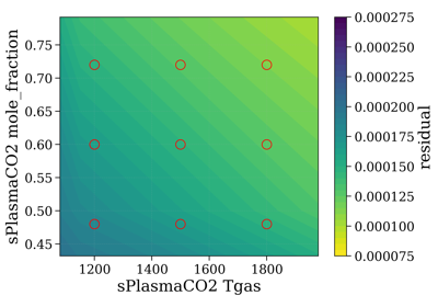
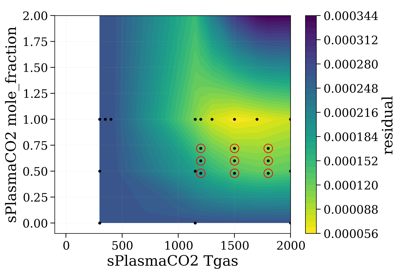
- precompute_residual(Slablist, xspace='database', yspace='database', contour='contourf', normalize=False, normalize_how='max', vmin=None, vmax=None)[source]
Plot residual for all points in database.
- Parameters
Slablist (configuration)
xspace (array, or ‘database’) – values of points to precompute. If ‘database’, residual is calculated for all points in database. Default ‘database’.
yspace (array, or ‘database’) – values of points to precompute. If ‘database’, residual is calculated for all points in database. Default ‘database’.
- Other Parameters
vmin, vmax (float) – used for colorbar
Examples
When
yparamis mole_fraction and we want to calculate for many mole fraction conditions from 0 to 1.selectTool.precompute_residual(Slablist, normalize=normalize, yspace=np.linspace(0.1, 1, 10))
- class DynVar(slab, param, func=<function DynVar.<lambda>>)[source]
Bases:
objectTo allow dynamic (runtime) filling of conditions in SlabList
- Parameters
slab (str) – slab config name in Slablist. Note that
'self'in DynVar can be used to refer to the DynVar’s own slab. Ex:slabPlasma={ 'Trot':2000, 'Tvib':DynVar('self', 'Trot'), }
param (str) – param name in slab config dict
func (function) – function to apply. Default identity
Examples
 slbPostCO2 = {
         'db':db0,
         'Tgas':500,
         'db':dbp,
         'Tgas':1100,
         'path_length':0.7,
         'mole_fraction':0.35,
          }

 slbPostCO = {
       'db':dbco,
       'Tgas':slbPostCO2['Tgas'],
       'path_length':DynVar('sPostCO2', 'path_length', lambda x:x),
                     # evaluated at runtime using names in Slablist
       'mole_fraction':0.01,
        }

Slablist = {
          'sPostCO2': slbPostCO2,
          'sPostCO': slbPostCO,
          }
You can also use a function, for instance to maintain the equilibrium concentration in a fit on temperature:
from radis.tools.gascomp import get_eq_mole_fraction
get_co2_eq = lambda T: get_eq_mole_fraction('CO2:1', T, 1e5)
slbPlasmaCO2 = {
         'db':dbp,
         'Trot':1500,
         'Tvib':DynVar('self', 'Trot'),
         'path_length':0.025,
         'mole_fraction':DynVar('self', 'Trot', get_co2_eq),
         }
Here the CO2 Plasma slab is always evaluated with Tvib=Trot and x_co2 at chemical equilibrium with T=Trot.
- class FitRoom(Slablist, slbInteractx, slbInteracty, xparam, yparam, perfmode=False)[source]
Bases:
object- Parameters
perfmode (boolean)
if ``True`` we try to optimize calculation times (ex (minimized windows)
are not recalculated)
Examples
See also
CaseSelector,Grid3x3,MultiSlabPlot,SlabsConfigSolver,Overpopulator,SlitTool
- class Grid3x3(slbInteractx=None, slbInteracty=None, xparam='', yparam='', plotquantity='radiance', unit='mW/cm2/sr/nm', wunit='nm', normalizer=None, s_exp=None)[source]
Bases:
objectWhere the output of a
CaseSelectoris shown.Examples
See also
CaseSelector,MultiSlabPlot,SlabsConfigSolver,Overpopulator,FitRoom,SlitTool,When,use,plot_for_export()- calc_case(i, j, **slabsconfig)[source]
notice j, i and not i, j i is y, j is x? or the other way round. It’s always complicated with indexes anyway… (y goes up but j goes down) you see what i mean it works, anyway
- plot_case(i, j, ax_out=None, plot_all_labels=False, **slabsconfig)[source]
notice j, i and not i, j i is y, j is x? or the other way round. It’s always complicated with indexes anyway… (y goes up but j goes down) you see what i mean it works, anyway
- Other Parameters
ax_out (ax) – if None, plot to the GridTool. Else, plot to this ax (used for export)
plot_all_labels (bool) – force plot all labels
- plot_for_export(style='origin', cases=[], ls='-', lw=1, xlim=None, ylim=None, labelvar='xy', color=None, labelunit='K', cutwings=0, kwargs_exp={})[source]
Sum all center column in one case.
- Parameters
cases (list) – list of [(row, column)] to plot. If
Noneor [], use a vertical line, i.e.cases=[(1,1), (0,1), (2,1)]
ls (str (‘-’, ‘-.’, etc.), list, or dict) – if str, use the same. If list, rotate. If dict, use
casesas keys.the first one is plot in solid line, the others in alternate with ‘-.’, ‘:’, ‘-.’
- Other Parameters
labelvar (‘x’, ‘y’, ‘xy’) – which variable to add. default ‘xy’ Ex:
Tvib=, Trot=
Tvib=
Trot=
cutwings – see
plot_stack()kwargs_exp (dict) – parameters forwarded to
plot_stackto plot the experiment
- class MultiSlabPlot(plotquantity='radiance', unit='mW/cm2/sr/nm', normalizer=None, s_exp=None, nfig=None, N_main_bands=5, keep_highlights=False, show_noslit_slabs=True, show_slabs_with_slit=True, wunit='nm')[source]
Bases:
objectPlot the center case in
CaseSelectorby also showing emission and absorption separately, and all slabs- Parameters
…
N_main_bands (int)
show main emission bands in case an overpopulation tool is defined.
N_main_bands is the number of bands to show. Default 5.
keep_highlights (boolean)
if ``True``, delete previous highlights when generating new case. Keeping
them can help remember the last band position. Default ``False``.
show_noslit_slabs (boolean)
if ``True``, overlay slabs with non convoluted radiance / transmittance
show_slabs_with_slit (boolean)
if ``True``, slit is applied to all slabs before display (this does not
change the way the radiative transfer equation is solved)
- Other Parameters
wunit (‘nm’, ‘cm-1’)
Examples
See also
CaseSelector,Grid3x3,SlabsConfigSolver,Overpopulator,FitRoom,SlitTool- plot_all_slabs(s: radis.spectrum.spectrum.Spectrum, slabs)[source]
- plot_broken(style=['origin'], xlim=None, lw_multiplier=1, skip_exp_range=[], cutwings=0, verbose=True)[source]
Not used in Fitroom, but can be used by user to export / save figure with broken axes
- Parameters
xlim (tuple, or list of tuple) – if None, all range is plot. If tuple, only this range is plot. If list of tuple, broken axes are used. Only works for
fig0though. Not Implemented forfig1.- Other Parameters
lw_multiplier (float) – multiply line widths
skip_exp_range ([(wmin, wmax), (wmin2, wmax2), etc.]) – dont plot these ranges for experimental spectrum. Default []
cutwings – see
plot_stack()
Examples
fig0 = slabsTool.plot_broken()
fig0.savefig('...')
- plot_for_export(style=['origin'], lw_multiplier=1, skip_exp_range=[], cutwings=0, figsize=[(20, 4), (20, 6.5)])[source]
Not used in Fitroom, but can be used by user to export / save figures
- Other Parameters
lw_multiplier (float) – multiply line widths
skip_exp_range ([(wmin, wmax), (wmin2, wmax2), etc.]) – dont plot these ranges for experimental spectrum. Default []
cutwings – see
plot_stack()
Examples
fig0, fig1 = slabsTool.plot_for_export()
fig0.savefig('...')
- class Overpopulator(slab, levels='all', nfig=None)[source]
Bases:
object- Parameters
slab – slab to connect to. Must be a slab calculated with from_band source mode
Examples
See also
CaseSelector,Grid3x3,MultiSlabPlot,SlabsConfigSolver,FitRoom,SlitTool
- class SlabsConfigSolver(config, source=None, s_exp=None, plotquantity='radiance', unit='mW/cm2/sr/nm', slit=None, slit_options='default', crop=None, retrieve_mode='safe', verbose=True, retrieve_error='ignore')[source]
Bases:
objectMachinery related to solving a specific Slabs configuration: parse the database, get the correct slab input, then calls the appropriate functions in neq.spec engine
- Parameters
config (dict) – list of Slabs that represent the Spatial model (to solve RTE)
source (‘database’, ‘calculate’, ‘from_bands’) – Whether to calculate spectra from scratch, retrieve them from a database, or combine vibrational bands Mode can be overriden by a ‘source’ parameter in every slab
s_exp (
Spectrum) – experimental spectrumplotquantity (‘radiance’, ‘transmittance_noslit’, etc.)
- Other Parameters
get_closest (bool) – when retrieving spectra from database, get cloest if set to True. Else get unique.
slit_options –
if
'default', use:{'norm_by':'area', 'shape':'triangular', 'unit':'nm', 'verbose':False}
and adapt
'shape'to'trapezoidal'if a tuple was given for slitcrop (tuple, or None) – if not
None, restrain to the given fitted interval.retrieve_error (‘ignore’, ‘raise’) – if Spectrum cannot be calculated or retrieved from Database, then returns
Noneas a Spectrum object. The rest of the code should deal with it. Else, raises an error immediatly.retrieve_mode (‘safe’, ‘strict’, ‘closest’) –
how to retrieve spectra when reading from database:
if ‘strict’, only retrieve the spectra that exactly match
the given conditions (allow scaling path_length or mole_fraction, still)
if ‘safe’, requires an exact match for all conditions (as in
‘strict’), except for the 2 user defined variable conditions
xparamandyparamif ‘closest’, retrieves the closest spectrum in the database
Warning
‘closest’ can induce user errors!!!. Ex: a Trot=1500 K spectrum can be used instead of a Trot=1550 K spectrum if the latter is not available, without user necessarily noticing. If you have any doubt, print the conditions of the spectra used in the tools. Ex:
for s in gridTool.spectra:
    print(s)
Examples
- calc_slabs(**slabsconfig) Union[radis.spectrum.spectrum.Spectrum, dict][source]
- Parameters
slabsconfig – list of dictionaries. Each dictionary as a database key
dband as many conditions to filter the database
- get_residual(s: radis.spectrum.spectrum.Spectrum, normalize=False, normalize_how='max')[source]
Returns difference between experimental and simulated spectra By default, uses
get_residual()function You can change the residual by overriding this function.Examples
Replace get_residual with new_residual:
solver.get_residual = lambda s: new_residual(solver.s_exp, s, 'radiance')
Note that default solver would be written:
from radis import get_residual
solver.get_residual = lambda s: get_residual(solver.s_exp, s,
                                             solver.plotquantity,
                                             ignore_nan=True)
- Parameters
s (Spectrum object) – simulated spectrum to compare with (stored) experimental spectrum
normalize (bool) – not implemented yet # TODO
Notes
Implementation:
interpolate experimental is harder (because of noise, and overlapping) we interpolate each new spectrum on the experiment
- class SlitTool(plot_unit='nm', overlay=None, overlay_options=None)[source]
Bases:
objectTool to manipulate slit function
- Parameters
plot_unit (‘nm’, ‘cm-1’)
overlay (str, or int, or tuple) – plot a slit in background (to compare generated slit with experimental slit for instance)
Examples
See also
CaseSelector,Grid3x3,MultiSlabPlot,SlabsConfigSolver,Overpopulator,FitRoom- plot_slit(w, I=None, waveunit='', plot_unit='same', wover=None, Iover=None)[source]
Variant of the plot_slit function defined in slit.py that can set_data when figure already exists
Plot slit, calculate and display FWHM, and calculate effective FWHM. FWHM is calculated from the limits of the range above the half width, while FWHM is the equivalent width of a triangular slit with the same area
- Parameters
w, I (arrays or (str, None)) – if str, open file directly
waveunit (‘nm’, ‘cm-1’ or ‘’)
plot_unit (‘nm, ‘cm-1’ or ‘same’) – change plot unit (and FWHM units)
warnings (boolean) – if
True, test if slit is correctly centered and output a warning if it is not. DefaultTrue